

Algoritmi di Neuroimaging per il Clustering di Traiettorie GPS
L’utilizzo di massa di dispositivi portatili come smartphone e smartwatch ci permette di avere uno storico completo della nostra vita. Grazie alle informazioni collezionate da questi terminali, riusciamo a ricostruire, con accuratezza estrema, lo storico dei nostri spostamenti.
L’applicazione di algoritmi di machine learning ai dati di posizionamento, ci permette di poter estrarre informazioni molto rilevanti utili a capire i nostri comportamenti. Alcuni di questi pattern sono ad esempio: il percorso che facciamo da casa a lavoro, le gite fuoriporta, quali locali frequentiamo il sabato sera etc..
In questo articolo descriveremo un efficiente e pratico algoritmo non supervisionato di machine learning per poter effettuare l’identificazione di pattern di traiettorie. Nella prima parte descriveremo l’algoritmo di clustering utilizzato per poter scoprire pattern, nella seconda invece mostreremo come realizzare concretamente tale algoritmo in Python.
Un Algoritmo di Neuroimaging per il Clustering di Traiettorie GPS
Invece di utilizzare i classici algoritmi di clustering come KMeans o DBSCAN, in questo articolo utilizzeremo un algoritmo di cluster comunemente utilizzato nell’analisi di immagini cerebrali.
QuickBundle (QB) (https://www.ncbi.nlm.nih.gov/pmc/articles/PMC3518823/pdf/fnins-06-00175.pdf) è un semplice e compatto algoritmo di clustering utilizzato per clusterizzare le fibre di materia bianca del cervello estratte tramite l’applicazione di algoritmi di trattografia (https://en.wikipedia.org/wiki/Tractography).
Da una semplice osservazione delle immagini mostrate qui di seguito, possiamo facilmente notale che le traiettorie GPS sono molto simili alle fibre di materia bianca.
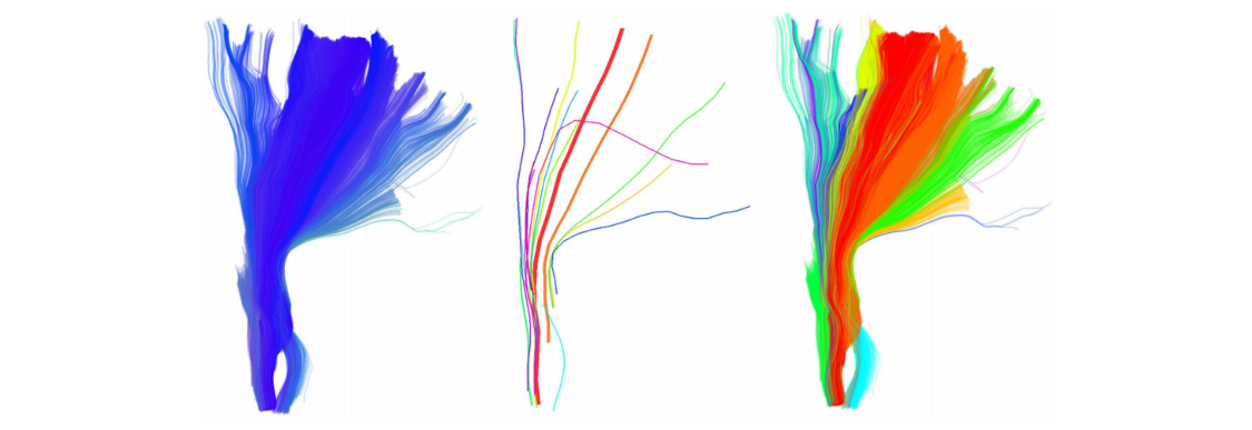
Figura 1 Esempio di fibre di sostanza bianca ottenute tramite algoritmo di trattografia.
Immagine da https://www.ncbi.nlm.nih.gov/pmc/articles/PMC3518823/pdf/fnins-06-00175.pdf
L’idea principale è quella di trattare una singola traiettoria GPS come una fibra di sostanza bianca e dunque unire nello stesso cluster traiettorie “simili”. Nel resto di questo articolo dunque assumeremo che Traiettoria GPS = Fibra di materia bianca.
Un esempio che mostra come l’algoritmo sia capace di raggruppare fibre in base alla loro traiettoria spaziale, è visibile nella seguente immagine.
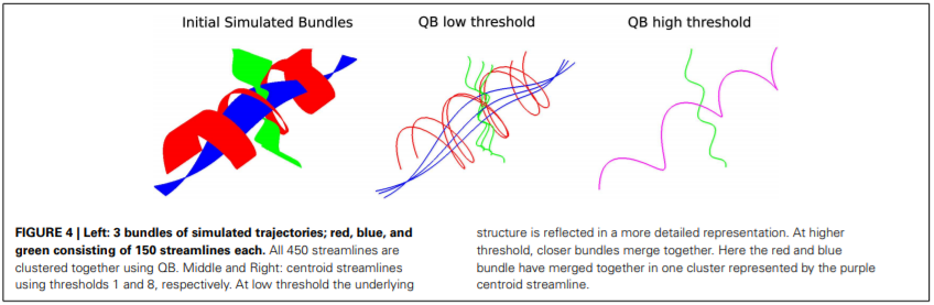
Figura 2 QuickBundle centroids with different thresholds. Imagine da Garyfallidis et al. Frontiers In Neuroscience, vol 6, 2016.
Aggiustando il parametro di threshold è infatti possibile raggruppare fibre più o meno distanti in accordo alla loro forma. Poiché il comportamento dell’algoritmo di clustering è fortemente dipendente dal valore assegnato al parametro di threshold, in contesti applicativi reali è necessario effettuare un tuning di questo parametro.
Altro risultato interessante ricavabile dall’algoritmo è legato alla capacità di generare un centroide caratteristico delle traiettorie aggregate in un dato cluster. Grazie a tale centroide è infatti possibile ottenere una rappresentazione compatta di un gruppo di traiettore.
Clustering delle Traiettorie GPS in Python
Vediamo ora come utilizzare praticamente, tramite linguaggio Python l’algoritmo precedentemente descritto su un dataset reali di traiettorie GPS.
I dati utilizzati in questo articolo sono relativi al tracciamento giornaliero degli spostamenti di un dato soggetto. Il dataset, rilasciato da Microsoft Research è disponibile al seguente link (https://www.microsoft.com/en-us/download/details.aspx?id=52367). Mentre una sua descrizione più approfondita è disponibile qui (https://yidatao.github.io/2016-12-23/geolife-dbscan/)
Prima di effettuare un’analisi approfondita dei dati, effettuiamo un plot delle coordinate GPS su google map utilizzando la libreria gmplot (https://github.com/vgm64/gmplot).
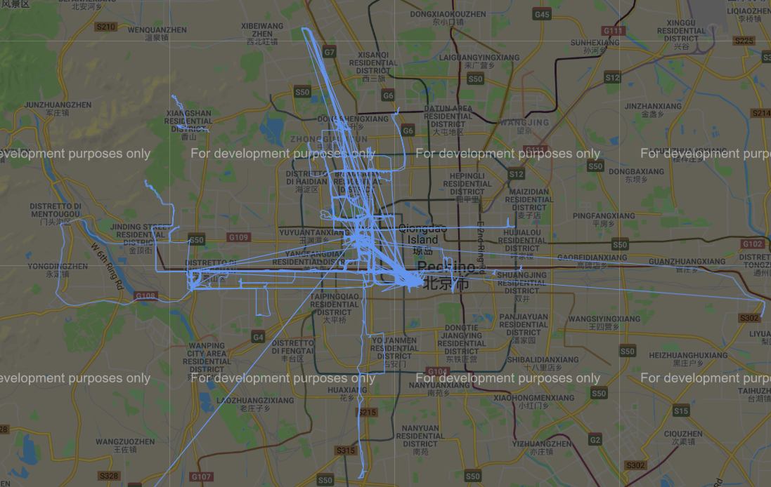
Figura 3 Traiettorie GPS nel dataset
Iniziamo dunque creando una funziona di distanza che tenga in conto del fatto che le traiettorie sono composte da coordinate GPS come descritto nell’immagine seguente.
Figura 4 Codice per calcolare le distanza tra coordinate GPS nelle traiettorie
Il codice calcola dunque la distanza tra tutte le coppie di punti all’interno delle traiettorie. E’ da notare che tale distanza può essere calcolata se e solo se le traiettorie hanno tutte un numero uguale di punti. Modificare tale porzione di codice affinché permetta di calcolare distanza anche tra traiettorie formate da punti diversi non è complesso.
Una volta definito come l’algoritmo QB deve calcolare la distanza tra i punti delle traiettorie, possiamo lanciare tale algoritmo sui dati di riferimento come descritto nella seguente immagine.
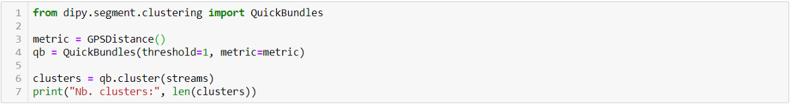
Figura 5 Codice Python per eseguire l’algoritmo di clustering
Possiamo dunque, sempre tramite l’ausilio di gmplot, rappresentare graficamente i diversi cluster ottenuti dall’applicazione di tale algoritmo su google map come mostrato nelle immagini qui di seguito.
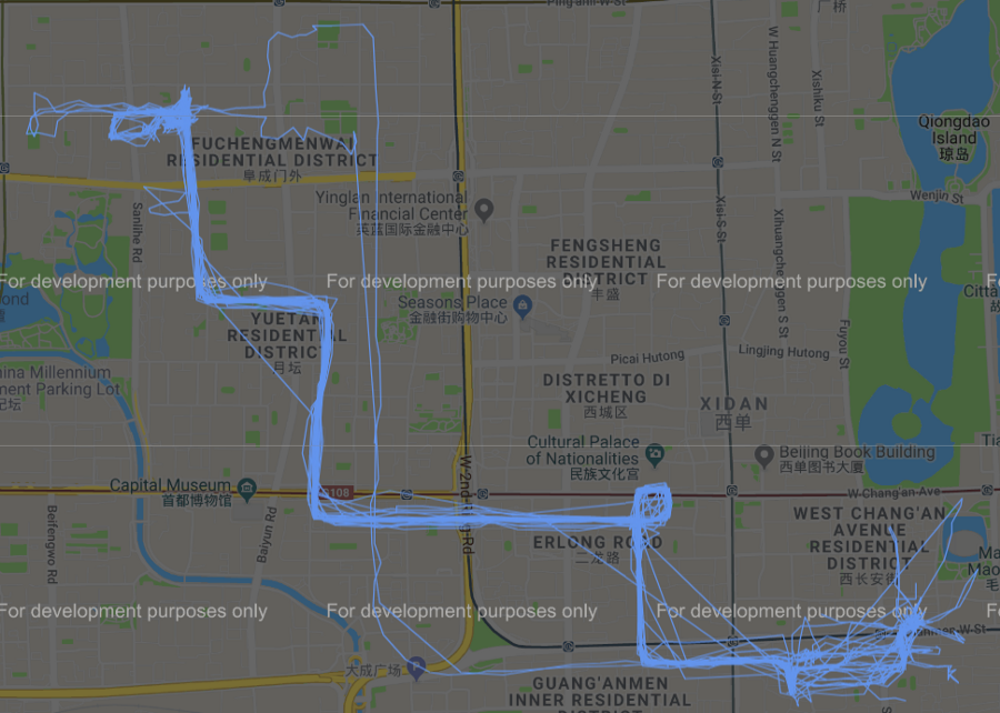
Figura 6 Cluster #0
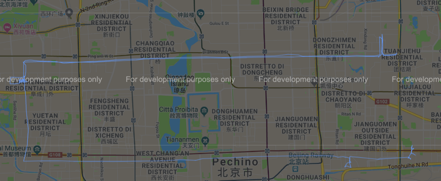
Figura 7 Cluster #2
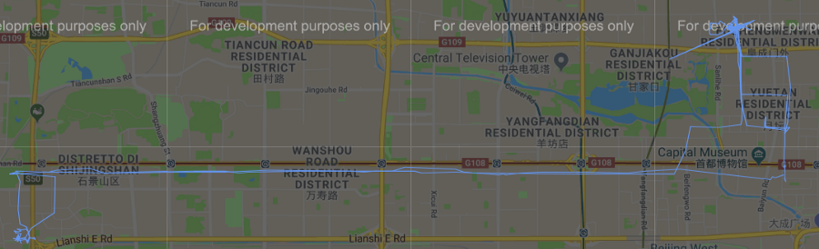
Figura 8 Cluster #30
Conclusione
In questo articolo abbiamo descritto un metodo semplice e veloce per clusterizzare traiettorie ottenute da rilevatori GPS. Al fine di raggiungere tale scopo abbiamo utilizzato un algoritmo non convenzionale utilizzato ampiamente nell’ambito nel neuroimaging.
La limitazione principale di questo algoritmo è legata alla scelta del parametro di threshold utilizzato. Tale problema però può essere facilmente risolto tramite un dettagliato processo di selezione.
Info su: https://medium.com/isiway-tech/gps-trajectories-clustering-in-python-2f5874204a53